


I. Introduction
Metamaterials can be best described as artificially designed structures to produce certain electromagnetic properties that do not exist naturally. Metamaterials with negative permittivity and negative permeability are called left-handed metamaterials (LHMs). LHMs have been extensively studied in the scientific and engineering communities. In 2003, LHMs were named one of the top ten scientific breakthroughs of the contemporary era by Science magazine. New applications, concepts, and devices have been developed by exploiting the unique properties of LHMs. The transmission line (TL) approach is an effective design method that can also analyze the principles of LHMs. Compared with traditional TLs, the most significant feature of metamaterial TLs is the controllability of TL parameters (propagation constant) and characteristic impedance. The controllability of metamaterial TL parameters provides new ideas for designing antenna structures with more compact size, higher performance, and novel functions. Figure 1 (a), (b), and (c) show the lossless circuit models of pure right-handed transmission line (PRH), pure left-handed transmission line (PLH), and composite left-right-handed transmission line (CRLH), respectively. As shown in Figure 1(a), the PRH TL equivalent circuit model is usually a combination of series inductance and shunt capacitance. As shown in Figure 1(b), the PLH TL circuit model is a combination of shunt inductance and series capacitance. In practical applications, it is not feasible to implement a PLH circuit. This is due to the unavoidable parasitic series inductance and shunt capacitance effects. Therefore, the characteristics of the left-handed transmission line that can be realized at present are all composite left-handed and right-handed structures, as shown in Figure 1(c).
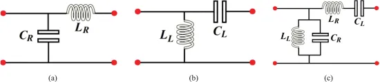
Figure 1 Different transmission line circuit models
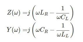
The propagation constant (γ) of the transmission line (TL) is calculated as: γ=α+jβ=Sqrt(ZY), where Y and Z represent admittance and impedance respectively. Considering CRLH-TL, Z and Y can be expressed as:
A uniform CRLH TL will have the following dispersion relation:
The phase constant β can be a purely real number or a purely imaginary number. If β is completely real within a frequency range, there is a passband within the frequency range due to the condition γ=jβ. On the other hand, if β is a purely imaginary number within a frequency range, there is a stopband within the frequency range due to the condition γ=α. This stopband is unique to CRLH-TL and does not exist in PRH-TL or PLH-TL. Figures 2 (a), (b), and (c) show the dispersion curves (i.e., the ω - β relationship) of PRH-TL, PLH-TL, and CRLH-TL, respectively. Based on the dispersion curves, the group velocity (vg=∂ω/∂β) and phase velocity (vp=ω/β) of the transmission line can be derived and estimated. For PRH-TL, it can also be inferred from the curve that vg and vp are parallel (i.e., vpvg>0). For PLH-TL, the curve shows that vg and vp are not parallel (i.e., vpvg<0). The dispersion curve of CRLH-TL also shows the existence of LH region (i.e., vpvg < 0) and RH region (i.e., vpvg > 0). As can be seen from Figure 2(c), for CRLH-TL, if γ is a pure real number, there is a stop band.
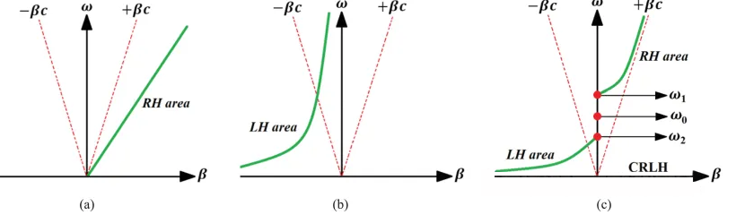
Figure 2 Dispersion curves of different transmission lines
Usually, the series and parallel resonances of a CRLH-TL are different, which is called an unbalanced state. However, when the series and parallel resonance frequencies are the same, it is called a balanced state, and the resulting simplified equivalent circuit model is shown in Figure 3(a).

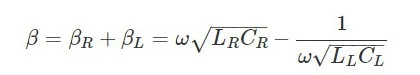
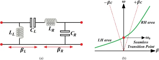
Figure 3 Circuit model and dispersion curve of composite left-handed transmission line
As the frequency increases, the dispersion characteristics of CRLH-TL gradually increase. This is because the phase velocity (i.e., vp=ω/β) becomes increasingly dependent on frequency. At low frequencies, CRLH-TL is dominated by LH, while at high frequencies, CRLH-TL is dominated by RH. This depicts the dual nature of CRLH-TL. The equilibrium CRLH-TL dispersion diagram is shown in Figure 3(b). As shown in Figure 3(b), the transition from LH to RH occurs at:
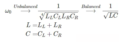
Where ω0 is the transition frequency. Therefore, in the balanced case, a smooth transition occurs from LH to RH because γ is a purely imaginary number. Therefore, there is no stopband for the balanced CRLH-TL dispersion. Although β is zero at ω0 (infinite relative to the guided wavelength, i.e., λg=2π/|β|), the wave still propagates because vg at ω0 is not zero. Similarly, at ω0, the phase shift is zero for a TL of length d (i.e., φ= - βd=0). The phase advance (i.e., φ>0) occurs in the LH frequency range (i.e., ω<ω0), and the phase retardation (i.e., φ<0) occurs in the RH frequency range (i.e., ω>ω0). For a CRLH TL, the characteristic impedance is described as follows:
Where ZL and ZR are the PLH and PRH impedances, respectively. For the unbalanced case, the characteristic impedance depends on the frequency. The above equation shows that the balanced case is independent of frequency, so it can have a wide bandwidth match. The TL equation derived above is similar to the constitutive parameters that define the CRLH material. The propagation constant of TL is γ=jβ=Sqrt(ZY). Given the propagation constant of the material (β=ω x Sqrt(εμ)), the following equation can be obtained:
Similarly, the characteristic impedance of TL, i.e., Z0=Sqrt(ZY), is similar to the characteristic impedance of the material, i.e., η=Sqrt(μ/ε), which is expressed as:
The refractive index of balanced and unbalanced CRLH-TL (i.e., n = cβ/ω) is shown in Figure 4. In Figure 4, the refractive index of the CRLH-TL in its LH range is negative and the refractive index in its RH range is positive.
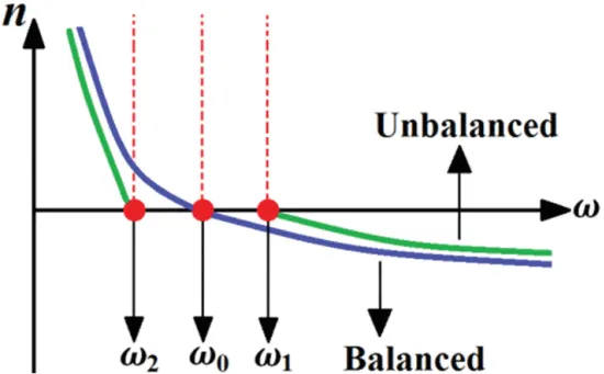
Fig. 4 Typical refractive indices of balanced and unbalanced CRLH TLs.
1. LC network
By cascading the bandpass LC cells shown in Figure 5(a), a typical CRLH-TL with effective uniformity of length d can be constructed periodically or non-periodically. In general, in order to ensure the convenience of calculation and manufacturing of CRLH-TL, the circuit needs to be periodic. Compared with the model of Figure 1(c), the circuit cell of Figure 5(a) has no size and the physical length is infinitely small (i.e., Δz in meters). Considering its electrical length θ=Δφ (rad), the phase of the LC cell can be expressed. However, in order to actually realize the applied inductance and capacitance, a physical length p needs to be established. The choice of application technology (such as microstrip, coplanar waveguide, surface mount components, etc.) will affect the physical size of the LC cell. The LC cell of Figure 5(a) is similar to the incremental model of Figure 1(c), and its limit p=Δz→0. According to the uniformity condition p→0 in Figure 5(b), a TL can be constructed (by cascading LC cells) that is equivalent to an ideal uniform CRLH-TL with length d, so that the TL appears uniform to electromagnetic waves.
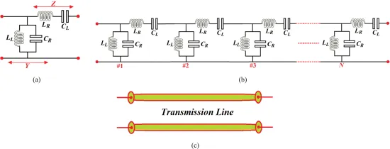
Figure 5 CRLH TL based on LC network.
For the LC cell, considering periodic boundary conditions (PBCs) similar to the Bloch-Floquet theorem, the dispersion relation of the LC cell is proved and expressed as follows:
The series impedance (Z) and shunt admittance (Y) of the LC cell are determined by the following equations:
Since the electrical length of the unit LC circuit is very small, Taylor approximation can be used to obtain:
2. Physical Implementation
In the previous section, the LC network to generate CRLH-TL has been discussed. Such LC networks can only be realized by adopting physical components that can produce the required capacitance (CR and CL) and inductance (LR and LL). In recent years, the application of surface mount technology (SMT) chip components or distributed components has attracted great interest. Microstrip, stripline, coplanar waveguide or other similar technologies can be used to realize distributed components. There are many factors to consider when choosing SMT chips or distributed components. SMT-based CRLH structures are more common and easier to implement in terms of analysis and design. This is because of the availability of off-the-shelf SMT chip components, which do not require remodeling and manufacturing compared to distributed components. However, the availability of SMT components is scattered, and they usually only work at low frequencies (i.e., 3-6GHz). Therefore, SMT-based CRLH structures have limited operating frequency ranges and specific phase characteristics. For example, in radiating applications, SMT chip components may not be feasible. Figure 6 shows a distributed structure based on CRLH-TL. The structure is realized by interdigital capacitance and short-circuit lines, forming the series capacitance CL and parallel inductance LL of LH respectively. The capacitance between the line and GND is assumed to be the RH capacitance CR, and the inductance generated by the magnetic flux formed by the current flow in the interdigital structure is assumed to be the RH inductance LR.
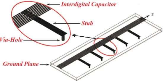
Figure 6 One-dimensional microstrip CRLH TL consisting of interdigital capacitors and short-line inductors.
To learn more about antennas, please visit:
Post time: Aug-23-2024


